Using the Yield Curve Generator

This chapter provides an overview of yield curves and discusses how to:

• Load source data for the Yield Curve Generator.

• Set up the Pricing Index Model.

• Set up market issues.

• Set up curve sets.

• Set up curve interpolants.

• Set up discount rates.

• Set up deterministic models.

• Generate yield curves.

• View yield curves.

See Also

Using the Interest Rate Modeler

Understanding Yield Curves

Yield Curves incorporate data from various market sources, such as Bloomberg, Reuters, and Telerate, by using the Extract-Transform-Load (ETL) process. You can use the ETL process to use user-defined source data for developing yield curves. You can specify the origin of the source data, define generic bond market volatility, credit spread, currency source data, and identify the type of data that you use to create the curves. Once you specify the source data for your curves, you then specify the curve interpolation methods to define how to interpret the source data.

There are two engines used to define yield curves, the Curve Generator application engine and the Curve Evaluator application engine.

The Curve Generator component enables you to set up the rules for interpolating a set of data points. Once you establish the setup rules, you can add, modify, or delete these rules. You do not need to set up new rules each time the Curve Generator component processes information.

The Curve Evaluator component is a process called by other support modules. This component is an online module that calculates rates as requested by other FSI applications. When the Curve Evaluator application engine receives a set of parameters from the calling application, the Curve Evaluator application engine calculates the requested rates and returns them to the calling application.

Common Concepts

The pages used to set up Yield Curves all share common concepts. This section discusses those concepts:

• Curve interpolation.

• Bootstrapping.

• Short-term yields.

• Issue types and frequencies.

• Derived data.

Curve Interpolation

The Curve Generator application engine supports the following interpolation methods:

• Hermite cubic: Creates a sequence of cubic equations between each data point.

  These cubic equations are controlled by the change in the curve at the two end points.

• Cubic spline: Creates a set of cubic equations like the hermite cubic, but the cubic spline guarantees that both the change in the curve and the rate of change at the quoted points (the slope and curvature of the function) remain constant.

  If you select this interpolation type, you need to further specify the way that the spline curve handles the left and right end points of each data set. This is done by modifications to individual equations that comprise the contiguous segments of the yield curve. Options are:

  • Continuous curl: The change in curvature, or curl, is made continuous between the first and second, and penultimate and last points of the data set.

  • Curvature constraint: Describes the behavior of the graphed point over the domain, enabling you to specify the degree of curvature at the first and last points of the data set.

  • Slope constraint: Enables you to specify the slope at the endmost points.

• Linear segments: Creates straight lines between each succeeding pair of quoted yields.

• Step function: Creates a yield curve from a given data point that looks like horizontal line segments.

  Until specifying a new yield, the step function uses the exact same yield for all subsequent maturities. This function can be very useful when referencing the prime rate because it has no maturity component. The Step function ignores the current term structure, therefore, no meaningful term information can be derived from it.

Interpolations are used on the Derived Data page and more specifically on the curve interpolation pages.

Bootstrapping

Using a technique called bootstrapping, the Curve Generator can take a coupon that is bearing market issue, strip its future cash flows (coupon payments) and convert them into a set of zero-coupon bearing market issues. To initiate bootstrapping, assign a coupon frequency to the coupon that is bearing market issue. If you do not select a coupon frequency value in the Market Issues page, the Curve Generator assumes that the market issue is non-coupon bearing. Once you set up the appropriate data in the Market Issues page, the Curve Generator can interpret the differences between zero-coupon market yields and coupon-paying yields.

Short-Term Yields

You must specify an overnight or short-term yield if you need rates from a given yield curve within maturities that are shorter than those that are in the source data. For example, source information from the data set includes a 30-day maturity point that is given by a treasury bill. However, when you require a term structure that includes maturities for overnight, two days, three days, one week, and so on, you must define those points with data that you determine is appropriate for those points. The Overnight Fed Funds is a commercial rate that is available if you do not have an in-house funding curve with a more desirable set of data points for defining those short-term maturities.

Issue Types and Frequencies

You define issue types and frequencies on the Market Issues page. The issue types and frequencies available for use are as follows:

• Singular issues: When the issue type is singular, the pricing information for the exact instrument that the CUSIP code designates becomes active and is later used for data set information.

  Singular issues do not have a predefined issue calendar and typically are nonstandard financial instruments. For example, bank notes are short-term money-market debt instruments that are issued in various denominations and maturities. Each bank note has a unique value, and the institution attaches a CUSIP code to track it.

• Repeating issues: The most recent issuance (also called on the run issuance) for a market issue is used to designate the data set point.

  Repeating issues have an anticipated frequency. For example, treasury notes have standard value and maturity, and they use the most recently issued instruments when building a yield curve. If you specify the market issue as a repeating issue, you must also set up an issue frequency and nominal tenor.

• Issue frequency: Indicates the periodicity for the issuance (for example, 52-week treasury bills are issued every 30 days).

• Nominal tenor: A surrogate tenor.

  Periodically organizations offer new security issues for notes and bonds. The nominal tenor acts as a surrogate tenor for these products according to their properties. A treasury bill, for example, may have an actual maturity of 28 days from issuance, but the nominal tenor assigned to this product may be 30 days. This facilitates the construction of term structures such as the Treasury Curve.

Derived Data

Derived data creates composite curves from multiple sources. Use the Derived Data page to define curves that are derived from operations performed on multiple curves. For example, you might define a term structure of credit spreads as the difference between a term structure of corporate bonds and the risk-free curve.

Alternatively, you can create curves by performing operations on two or more existing curves and designating the interpolation method that provides the desired result. For example, you can create a term structure by averaging the LIBOR and CD yields to comprise the overnight to two-year rates and arrive at the two-to-ten-year rate by using treasury notes and positively shifting by 150 basis points. By including the 30-year treasury bond rate, you can complete construction of the newly defined curve. A credit spread curve can be constructed by subtracting the risk-free curve from a curve that is composed of corporate bonds.

Note. The risk free curve is typically defined by the Treasury Curve. You can define the risk-free curve according to your business practices.

• The lag frequency defines a historic period of time when you want your calculation to begin.

  The lag frequency period is not included in the rolling average interest rate calculation unless the value is set to zero. For example, if today is February 2002, and you set the lag frequency to three months and the rolling average frequency to eight months, the application calculates the rolling average from November 2001 to April 2001. The lag period from February 2002 to December 2002 is not included in the interest rate calculation.

• A rolling average frequency defines the span of time that is being used to calculate a rolling average.

  The data within this time span is used to calculate the rolling average rates. Rolling averages are based on existing rolling average rates. A rolling average can only be calculated based on a previously defined data set.

Note. Since the Treasury Curve comprises issues varying in maturity from an overnight to a thirty-year bond, nominal tenors are specified for each treasury product that you want to use in constructing curves. This eliminates the need for an exact day count for each issue every time that you want to construct a yield curve.

Loading Source Data for the Yield Curve Generator

Typically, source data enters the application during the Extract Transform and Load (ETL) process. However, if you have market interest rates that do not need frequent updating or source data that you create, you can bypass the ETL process and enter these data sets manually. The Curve Generator application engine obtains the rates and maturities and processes them according to the defined data sets and interpolation methods.

Note. Do not modify data imported from a subscription service such as Bloomberg, Reuters or Telerate. Also, you cannot manually add information for composite source data.

Page Used to Load Source Data for the Yield Curve Generator

Entering the Yield Curve Data

Access the Yield Curve Dataset Entry page.

Select a currency code that you want to use for reporting purposes. Market issues such as LIBOR rates are reported in multiple currencies. Enter a yield. The yield is the market-determined yield to maturity at the time of analysis. Enter a coupon value to indicate the rate of return to the bearer for each interest coupon payment. Only when the Market Issue is non-coupon bearing should this rate be equal to zero and the price be equal to 100. Enter a price when the source data is a discounted financial product such as treasury bonds or corporate bonds. Indicate the quoted market price on a par 100 basis, or leave it blank. On the Generic Curve DataSet Entry page, enter x and y values to indicate the spread.

Setting Up the Pricing Index Model

This section provides an overview of the Pricing Index Model and discusses how to:

• Set up the Pricing Index Model.

• Adjust the Pricing Index.

• Define the Pricing Index step functions.

To set up global definitions for a particular pricing model, you need to create it within the Price Index Model, then specify which indices the model uses. You can do this on the Price Index page. The Price Index page enables you to define a target index that specifies the characteristics of the pricing rule. For example, you can define whether the target index behaves differently in declining rate environments versus rising environments or whether it is a smooth or step function. Also, the calculated value of the target index (as defined by the index equations) is validated against the key underlying rate for reasonableness. The adjusted target index is constrained by a range that is defined as a fixed spread against the key underlying rate.

Understanding the Pricing Index Model

An appropriate product rate forecast is necessary to capture reasonable interest rate spreads between future products and market rates (and between asset and liability products themselves) in all simulated rate environments. The Pricing Index Model enables you to model future product pricing rates by using market interest rates (for example, treasury, LIBOR, or derived yield curves) as inputs for user-defined product-pricing algorithms. Product rates can be derived in market or deterministic scenarios. The predicted rates can then be used:

• By the Cash Flow Generator application engine to calculate future product rates for variable rate products.

  The Cash Flow Generator uses these refinance rates (future product rates) to set the repricing rate on variable rate products and to ascertain the level of prepayment and deposit runoff. For example, the Cash Flow Generator uses the Pricing Index Model rates for calculation of future payment amounts on adjustable rate mortgages.

• By the Behavioral Models to calculate future prepay and runoff rates.

  These models use future product rates for the calculation of their respective prepayment or deposit runoff rates.

• To assign future product rates to forecasted volumes that are generated by Portfolio Forecast.

Use the Pricing Index Model to define indices upon which the rate that is paid or charged for an individual product is based. This may be as simple as identifying a single rate from a yield curve (for example, the seven-year CMT from the US Treasury curve) or a combination of rates from different yield curves. You can include other defining variables, such as a lag component or the addition or subtraction of rate spreads in the model.

The Pricing Index Model is scenario aware. For example, if the index rate is calculated from a treasury rate and the treasury curve is shocked by 100 basis points, the Pricing Index Model uses the shocked value as its input. The only requirement is that you specify the appropriate rate assumption for the scenario definition. There is no need to redefine Pricing Index Models in order to run a shocked scenario impacting all product rates. (The supported scenarios are market and deterministic)

The Pricing Index Model can use the Function Evaluator for calculating formulas leading to assumptions in building pro forma financial statements.

This section discusses:

• Pricing Index Model definitions.

• Target index definition.

• Smooth and step functions.

• Index adjustments.

• Key underlying interest rates.

• Deltas.

Pricing Index Model Concepts

Whether you create a model from an index or a yield curve, you can define pricing models that behave differently in a rising rate environment and in a declining rate environment. For example, you can define a systematic widening (or narrowing) of spreads in a rising (or declining) rate environment. You also can define indices that respond continuously to the movement of the underlying interest rates or that move as a step function. The creation of a step function index models the pricing behavior of administered rates (that is, money market accounts, demand deposit accounts, and so forth). You can also define constraints in the pricing model that ensure reasonable spread relationships in extreme interest rate environments.

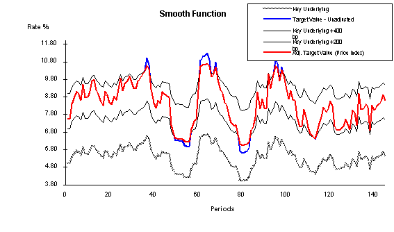
The following illustration represents these concepts. Here, the price index is evaluated against key underlying values in a smooth function. The unadjusted target value is evaluated against the key underlying rate for reasonableness. This test can be defined as a spread against the key underlying. This test ensures that the unadjusted target value never falls out of this reasonableness range, regardless of the absolute level of interest rates.

Price Index Concepts Illustrated

The red line (Adj. Target Value) is the most important to follow. This represents the price index after adjustments; it remains within a defined spread range from the key underlying value (for this example, they are set at +400 and +200 bp). In this case, the adjusted target value is the price index because the value remains within the defined constraints. The blue line represents the unadjusted target value before evaluation against the constraints. In the periods where there is no blue line visible, the red line and the blue line are equal and there is no constraint violation. Where the blue line is visible, it exceeds the constraints and therefore cannot be the price index. The gray line is the original key underlying value that does not have any constraints.

Target Index Definition

The Target Index page enables you to choose whether you want the target index to be defined as an equation or a single point from a specified yield curve. Target indexes that are defined from two separate equations can be defined for a rising rate environment and a declining rate environment, or one function can be used for both rate environments. The determination of whether to use the upward or downward equation is based on the change in the key underlying value. Options are Upward = Downward to create a single equation or Upward < > Downward to create two different equations for the respective change in direction. Use Single Point Index for creating a price index that is keyed to one rate from a specified yield curve.

Smooth and Step Functions

The Index Adjustment page enables you to assign a step function to the adjusted target index. Choose Smooth if you want a price index that continuously moves in response to the movement of the target index. Choose Step (for step function) if you want the price index to move only when the spread between the price index and the target index is in excess of a specific threshold for a defined period.

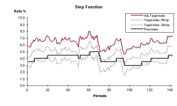
Movement of the step function is defined by the criteria in a range that you specify that affects a change in the price index value. The step function range is defined as a minimum and maximum spread relative to the adjusted target index. As long as the price index value stays within this range, it does not change. If the price index drifts below or above the range (for a consecutive period of time that is also defined by the user) it is adjusted upward or downward. The level of adjustment may be defined to be an absolute move or a percentage of the difference between the current rate and the target index. The following graph illustrates this concept:

Smooth and step functions

The solid, red line represents the price index (adjusted target index) that you define in the Price Index page after it is evaluated against the key underlying rate that is defined in the Index Adjustment setup page. The dotted lines represent the range that you define as the allowable spread between the Adjusted Target Index and the current index value (product rate). The solid, angular line is the way that the adjusted price index responds to the step range and adjusted target index.

Index Adjustments

The Index Adjustment page enables you to define the parameters that are evaluated against the target index for a reasonableness test.

The target index is the result of the equation or the single point rate as defined in the previous page. The target index may be based upon a single forward rate from a single yield curve, or it may be a blend of multiple rates from more than one yield curve. The target index is evaluated for reasonableness against a key underlying rate The target index changes as a result of changes in the equation parameters, however, sometimes certain changes can lead to values that are considered unrealistic. For example, the equation is defined as three-month LIBOR raised to the 1.25 power to capture an increased spread dynamic in higher rate environments. This might be fine when three-month LIBOR is 4 percent, returning a target index rate of 5.65 percent. However, this may not work well when three-month LIBOR is 8 percent, resulting in a target index of 13.45 percent. In this example, it may be desirable to ensure that the index is never greater than three-month LIBOR plus 300 basis points. The Index Adjustment page enables you to define the parameters that test the target index for reasonableness in all rate environments and constrain the value based on those tests.

Key Underlying Index Rates

(Appears only if you specify Index in the Key Rate Type field). Specify the type of key underlying index that you want. Index key rate types are available for you to set up adjustment curves instead of using market rates for target rate adjustments. For example, let's say that the benchmark for setting product rates is the Prime Rate or 11th District COFI (cost of funds index). These must be defined as an index because they are not market-traded rates or instruments that can be used to construct a yield curve. Consequently, if you want to ensure that the product rates (defined by a function) are always within a reasonable benchmark, this is how you accomplish that.

Note. An Index ID cannot be defined as the key underlying rate for itself.

Deltas

This field captures the rate change rule that is applied to the price index in a declining rate environment. This field may appear as Downward Delta (bp) or Downward Percent (%) depending on which option you chose in the Adjustment Method field. The downward delta is the basis point change subtracted from the price index if the threshold-interval test is true. The downward percentage is the relative basis point change subtracted from the price index if the threshold-interval test is true. It is calculated as a percentage of the spread between the price index and the target index.

Captures the rate change rule that is applied to the price index in a rising rate environment. This field may appear as Upward Delta (bp) or Upward Percent (%) depending on which option you chose in the Adjustment Method field. The upward delta is the basis point change added to the price index if the threshold-interval test is true. The upward percentage is the relative basis point change added to the price index if the threshold-interval test is true. It is calculated as a percentage of the difference between the price index and the target index.

Pages Used to Set Up the Pricing Index Model

Setting Up the Pricing Index Model

Access the Price Index page.

Note. This is a dynamic page. The options that you choose in the fields may activate or deactivate additional pages and fields.

Set up general price index information. Define the target index by choosing Upward <> Downward (for two equations), Upward = Downward (for one equation), or Single Point Index (for yield curve rate) in the Index Equation field. Select a curve function. Options are Smooth or Smooth & Step.

Set up specific target index information. These are the fields that may be displayed depending on the target index that you define:

If you define the target index by using equations, you need to set up the Index Adjustment page. (Skip this process if you use yield curves to define the index). If not, you can optionally enter setup notes in the Notes page.

Adjusting the Pricing Index

Access the Index Adjustments page.

On the Index Adjustment page, specify the type of key underlying value that you want the target index evaluated against by specifying a key rate type. Options are Yield Curve or Index.

• If you select Yield Curve, specify the corresponding yield curve code and maturity.

• If you select Index, specify the corresponding Index ID.

Then, enter values in basis points for the upper and lower boundaries of the target index spread in the maximum and minimum spread fields. Enter values in percentage points for the maximum and minimum rates of the target index over its entire life in the absolute maximum and minimum fields. When you are finished, set up the Step Functions page.

Defining the Pricing Index Step Functions

Access the Step Functions page.

Set up the Step Functions page for both equation and yield-curve defined target indices. Specify the upper and lower boundaries of the spread threshold in basis points. Do this in the Index <> Adj. Key Rt +- (bp) fields. Use the decrease column for upper boundaries and the increase column for lower boundaries. Values may be positive or negative.

In the For Consecutive Periods fields, specify the interval of consecutive periods for which the threshold test must be true to initiate a change in the price index (for both upper and lower boundaries).

In the Adjustment Method fields, indicate the manner in which the step function adjusts to fluctuations in interest rates and periods. Choose Delta for an absolute change or % of Difference for a relative change in the price index if the threshold test and the interval test are true.

In the Delta fields, specify the rate change rule that is applied to the price index in a declining (Downward Delta) or rising (Upward Delta) environment.

Setting Up Market Issues

This section discusses how to set up market issues.

Pages Used to Set Up Market Rules

Setting Up Market Issues

Access the Market Issues page.

To set up the Market Issues page, select a currency code, accrual basis code, and a decimal convention.

Then, select the issue type. If you select Singular, define a Maturity Date and a CUSIP Code. If you select Repeating, define an Issue Frequency and a Nominal Tenor.

Setting Up Curve Sets

This section provides an overview of operation codes and discusses how to:

• Define the curve sets data sources.

• Define the curve sets market issues.

• Define the curve sets derived data.

• Define the curve sets generic data.

To set up curve sets, set up the Data Source page. On this page, you specify the data type that you use. This data type field determines which of the following additional pages you set up:

• Generic Data page.

• Market Issues page.

• Derived Data page.

Understanding Operation Codes

Operation Codes are used to calculate new data based on existing data sets. These codes are used on the Derived Data page.

This chart illustrates some examples of operation codes:

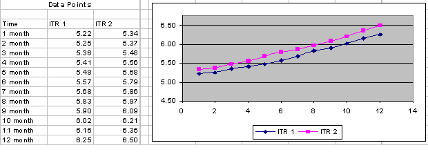
Operation codes

The operation codes are:

• Average (AVG)

• Also

• Difference (DIFF)

• Minimum (MIN)

• Maximum (MAX)

• Shift

• Shift Range

• Splice

• Sum

AVG

Average returns the average value between two values. For example, following is a plot of internal transfer rate 1 and internal transfer rate 2, with the average of the two data sets making up the third plot as the average of the two data sets:

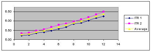
AVG

ALSO

Also adds a new source to an already calculated operation and repeats this calculation with the result of the previously calculated result and the new source. Also is most likely used in conjunction with the AVG operation code to average an additional data source with the previously averaged values.

For example, the ITR 1 curve and the ITR 2 curve are averaged by using the AVG operation code. In addition, you want to calculate the average between this newly calculated average (comprised of the averaged data set ITR 1 and ITR 2) and the Corp BB curves. This is done by using the ALSO operation code. The following graph illustrates the Also operation code:

(ITR 1 + ITR 2) /2 = Average value 
(Average + Corp BB) /2 = Also value 

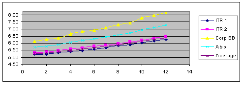
ALSO

Note. Average represents the average between ITR 1 and ITR 2. Also represents the average between average and Corp BB.

DIFF

The absolute difference between two yields. DIFF subtracts the lower from the higher value and displays the new value. No negative values can result from this operation.

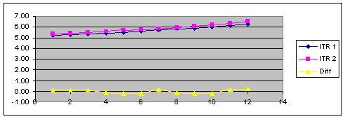
DIFF

MIN

The absolute minimum value from two sources. This operation code compares two data sets and selects the lowest representative data point between the two data sets.

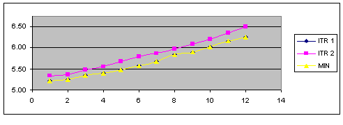
MIN

MAX

The absolute maximum value from two sources. This operation code compares two data sets and selects the greatest representative data point between the two data sets.

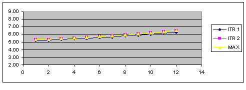
MAX

SHIFT

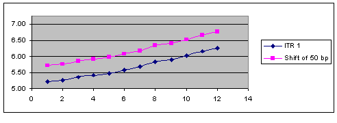
The SHIFT operation code allows the user to apply a basis point shift to an existing data set. The basis point shift is applied to the entire data set.

SHIFT

SHIFT RANGE

SHIFT RANGE allows the user to apply a basis point shift to an existing data set that is within a specified time frame. The time frame is specified with a start maturity and an end maturity, which are defined in days, months, or years rather than as actual dates.

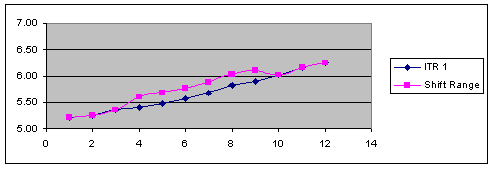
SHIFT RANGE

SPLICE

Splice divides an existing curve into a new curve with two or more data sources or types of interpolants.

Note. A curve's interpolant can only be spliced if the Global Interpolant is not checked.

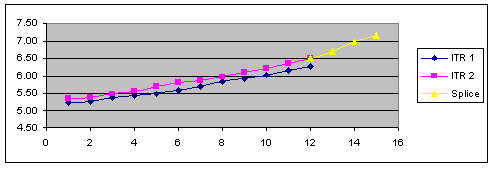
SPLICE

SUM

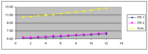
The SUM operation code adds the data points of two data sets and creates a third data set with the totals.

SUM

Pages Used to Set Up Curve Sets

Defining the Curve Sets Data Sources

Access the Data Source page.

Specify the type of data sets from which you construct the yield curves. Options are:

• Generic Data.

  The source data is composed of user-defined data. You supply the x-y axis coordinates and units of measure for this data.

• Market Issues (default).

  The market rate instrument data is assigned to this source data.

• Derived Data.

  Create your own data from more than one market source. Your choice determines the type of tab that follows the Data Source tab.

Specify the purpose for these data set points. Options are Yield Curve, Commodity, Credit Spread, Foreign Exchange, Volatility, or Other. Specify the currency code and the accrual basis code. Set up the second tab (subsequent Curve Sets page). This tab varies according to the selection in the Data Type field.

Defining the Curve Sets Market Issues

Access the Market Issues page.

Select a Market Issue Code where you are prompted. Choose from codes that you previously set up on the Market Issues page. Specifying a code in this field enables you to create a synthetic curve comprised of numerous market issues that have different attributes and assign those combined market issues to a new data source.

There is a minimum number of data points (market issues that you must select for the curve set definition) to generate unique curve results. This minimum number varies depending on the yield curve interpolation method: 1 for step, 2 for linear, 3 for hermite cubic, and 5 for cubic spline.

Defining the Curve Sets Derived Data

Access the Derived Data page.

To set up the derived data page, specify the source data that you want to use for this composite curve in the Start Data Source field. Should the construction of data points that you specify require more source data, select an interpolant to use in fitting a curve to the data points. Select the Global Interpolant check box to interpolate all the data in the new set in the same manner as the source data that you specify in the Start Data Source field.

If you want to calculate rolling averages based on historic interest rate information, check the Rolling Average box. This activates two other fields, the Lag Frequency and Rolling Average Frequency fields that enable you to select dates from previous yield curves.

Next, set up the curve operators. The Step # field indicates the source data that is affected by the chosen operation and helps you keep track of the operations that are performed and the segments of the composite curve that are impacted). Select an operation code to determine operation on the current (and possibly previous) data set that is given in the data source prompt box. Options are: Average, Also, Difference, Max Min, Shift, Shift-Range, Splice, and Sum. Depending on the selection, the following fields may appear:

Defining the Curve Sets Generic Data

Access the Generic Data page.

Enter values for the X and Y axis. These values are previously set up in PeopleSoft Enterprise Performance Warehouse by using the Unit of Measure page. Create generic data sets to provide maximum flexibility for curve generation of desired user defined parameters and data. You provide the data inputs and measures that are needed to define the data set.

Setting Up Curve Interpolants

This section discusses how to define curve interpolants.

Pages Used to Set Up Curve Interpolants

Setting Up the Curve Interpolants

Access the Curve Interpolants page.

Select a Data Set Code and Equation Type. This grid tells the Curve Generator how to use the equation to calculate curves. Different interpolation algorithms can be used for different sections of the curve set.

1. Specify the Tenor and UOM (unit of measure). If you need rates from a given yield curve within maturities that are shorter than those that are in the source data, indicate an overnight or short-term rate. This enables Curve Generator to interpolate the required values between the overnight or short-term rate and the selected source data.

2. Specify the curve interpolation method that you want to define. Options are: Cubic Spline, Hermite Cubic, Linear Segment, or Step Function.

3. Indicate where you want terms to be spliced by defining the boundary. If the tenor that you specify in a grid does not land on a data point, this field enables you to specify an alternate point to use (closest, prior, or behind).

4. If you define this equation as a cubic spline interpolation, the Spline Option column appears. Specify the way that you want the spline curve to handle the left and right endpoints of each curve set. Options are: Continuous Curl, Curvature Curl, Curvature Constraint or Slope Constraint.

5. Select specific values for the slop or curvature at the left and right points, known as the constraints. If you define the spline option as a continuous curl, you do not need to set up the right constraint.

6. If you specify this equation as a slope constraint, set up the estimates for left and right constraints.

Setting Up Discount Rates

Define discount factors when calculating the net present value (NPV) on a set of cash flows.

See Using the Interest Rate Modeler.

Setting Up Deterministic Models

This section provides an overview of deterministic scenarios and discusses how to:

• Set up the deterministic model.

• Set up the shock model.

• Set up the drift model.

Understanding Deterministic Scenarios

The Deterministic Interest Rate Scenario Generator enables you to model an organization's exposure to interest rate risk. There are two general (deterministic) methods for modeling interest rate movements.

• The Rate shock (shock model) enables you to model instantaneous changes to the market yield curve in an arbitrage-free scenario.

• The Rate ramp. (drift model) employs the option allowing individual tenors on a yield curve to move gradually and independent of one another over a specified period of time. The drift model does not ensure an arbitrage-free environment.

Shock Model

The shock model is an example of an arbitrage-free scenario that you can employ to model the financial institution's sensitivity to interest rate changes on the NPV of a portfolio. Use the entire yield curve (term structure) to ascertain the appropriate discount factors for future cash flows determined by the portfolio's makeup of on-balance sheet and off-balance sheet items. Use two methods for defining scenarios.

• The parallel shift method enables you to define an instantaneous change to the term structure. As a result of this shock, each point of the term structure is changed by the same amount.

• The shaped curve method is also an instantaneous change but it enables you to define the new shape of the curve.

In this manner, the scenarios allow for things like twists, steepening of curves, flattening of curves, and so on. Included in shock model functionality is the ability to select different shock assumptions for different yield curves. This enables you to determine the sensitivity analysis for basis risk (For example, two yield curves that move in different fashions).

Regulators require financial institutions to illustrate the impact on their portfolios due to adverse rate changes. This is accomplished by subjecting the current portfolio to a series of rate shocks (For example, immediate rate changes of 100-400 basis points). This technique illustrates both the earnings that are at risk and the value that is at risk for a financial institution's portfolio. These techniques are effective tools for both monthly review of the entire organization's book and daily analysis of smaller trading books. Regulators require that the financial institution's risk capital be sufficient to withstand a rate shock scenario. Although an actual market rate shock is unlikely, the shock model does provide a relative measure of the financial institution's risk exposure while satisfying regulator's requirements.

Drift Model

Use the drift model method to model net interest income (NII). NII focuses on the spread between income from financial products that are offered and the match funded liabilities. The Drift Model method enables you to independently define future values of assorted tenors from the same yield curve.

Arbitrage-free forward rates are not calculated in drift models. This is useful for creating inverted yield curves or modeling gradual changes to the term structure, curve twists, and curve shifts (nonparallel shifts).

Note. It is assumed that the analyst conducts the analyses with the understanding that the specified series of term-structures are no longer arbitrage-free with respect to the current term-structure.

Pages Used to Set Up Deterministic Models

Setting Up the Deterministic Model

Access the Model Definition page.

Specify this model to be either a shock model or a drift model.

• If you selected a shock model, enter the value of interest rate shock in basis points in the Shock (bp) field. For example, 100 indicates a 100 basis-point shift upward in rates for the selected yield curve. Likewise, -100 indicates a 100 basis-point drop in rates to the selected yield curve. Then, click the All button to apply the shock value to all data set codes in the grid. The default value is of a parallel shift yield.

• If you select a drift model, enter the schedule (daily, monthly, or yearly) for which future yield curves are built. Enter values up to five digits. All three fields cannot be left blank. When the rule is processed, the number of daily time steps is first considered, then the monthly time steps, then yearly.

Next, enter the model specifications. Fields that may appear are:

Setting Up the Shock Model

To access this page, ensure that the model is defined as a shock model in the Model Definition page and then click the Tenors button.

You supply the change to the rate in basis points next to the designated tenor shift. As you supply the Delta (bps) (delta basis points) values, the instantaneous yield curve shift scenario that is plotted in green is charted alongside the base scenario plot. You have the flexibility of designating shaped shift types (besides a parallel shift) across all tenors. Click the Reset button to reset the curve shift scenario plot and data points. Click OK to accept the changes to the shock model.

Setting Up the Drift Model

To access this page, ensure that the model is defined as a drift model in the Model Definition page and then click the Tenors button.

Set up the Market Issues that enable you to establish which data points you want to plot. Specify source data in the Data Point field. Include or exclude data points using the Plot check box. Click the Reset button to clear all the selected data points. Use Order to change the order of the data points that are plotted.

The Futures Rate Changes group box enables you to establish the future rate movements of the data points that you set up in the Market Issues group box. Select data points to which you want to apply future rate changes. Then, establish a future period by using the Future Period and UOM (unit of measure) fields and enter the basis point change in the Delta (bps) field.

Click OK to accept the changes.

You also have the option of creating a parallel shift in the drift model by using the data points that you previously selected on the Include Market Issue grid. Just select the period of time that you want to apply the shift in the Parallel Shift group box (rather than creating a series individual future period points in the Future Rate Changes group box) and indicate the value of the aggregate move in basis points. This shift applies to all data points that you previously selected on the Include Market Issue grid. Then, click the Apply button.

Click the Graph button to generate a graphical representation of the drift model.

Generating Yield Curves

This section discusses how to generate yield curves and drift yield curves.

At this point, you've set up all the relevant pages for yield curves. Your next step is to create yield curves. You do this by running a jobstream that includes the Curve Generator application engine in its processing. Creating yield curves is an iterative process. If you don't think the output is satisfactory, you can go back to the various setup steps that are outlined in this chapter and change the specifications as needed. Then, you can run the jobstream again and review the results.

To help you review your yield curves, you can use:

• The View Curves inquiry page that enables you to graphically view the yield curve that you created.

• Crystal reports, for further analysis.

Note. Ensure that the data is up-to-date. You can do this by checking the as of dates in the pages before generating the yield curves. The Pricing Index Model uses information from Curve Generator that if incorrect, negatively affects processing.

Pages Used to Generate Yield Curves

See Also

Understanding Common PeopleSoft Financial Services Industry Processes

Generating the Drift Yield Curves

Access the Drift Generation page.

To generate drift models, ensure that you set up the drift models, then process that model by using the Drift Generation page. The Drift Generation page is a run control page that creates drift models that are established with drift yield curves. Select the drift model that you want to process in the Term Structure Model field, select a Curve Date, and click the Run button.

Note. Unlike drift rates, which need to be calculated by the Drift Generator, the shock rates need no prior generation. They are calculated at run time by the cash flow generator.

Viewing Yield Curves

Yield curves are constructed and stored in the database as ranges of maturities for which a single cubic equation (y = a + bx + cx² + dx³) describes the yield curve through those maturities. A complete yield curve for maturities from zero through thirty years or longer is typically made up of a few of these equations, each describing a segment of the curve. You can use the equations making up the complete curve in a spreadsheet for graphing purposes. Individual forward rates can be calculated online by using this page.

Page Used to View Generated Yield Curves

Viewing the Generated Yield Curves

Access the View Yield Curves page.

To view yield curves, enter a value in the Maturity field. Enter a data in the Maturity Dt field. Today's date is the default. Click the Calculate button next to the Maturity field. The rate appears in the Rate field. Click the Graph button to graph the values. A grid appears, showing a graphical representation of the yield curves.