Using the Statistical Matrix
This topic provides an overview of the statistical matrix.
The statistical matrix is a spreadsheet view of various statistics that you can customize to include any statistic that Quality calculates. You can display the statistics in various formats.
Some statistics may be altered through the use of non-normal distribution assessment techniques. Quality incorporates the following methods to achieve an appropriate distribution fit. Both methods use the Pearson family of distributions.
A test of normality, using the skewness and kurtosis of the distribution.
If the distribution is normal at a 95 percent confidence, then the data is evaluated based on the normal assumption. If the distribution isn't found to be normal at a 95 percent confidence, then the data is evaluated using the Pearson Best-Fit family of curves. This is the recommended method if you are unsure of the distribution type.
Direct use of the Pearson Best-Fit family of curves.
The routines determine the best-fit and adjust the statistics appropriately.
The set of basic statistics includes measures of central tendencies, measures of dispersion, and the other descriptive statistics, as shown in the following table:
|
Equation |
Statistic |
Alternate Equation Forms |
|---|---|---|
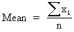
|
The mean is the arithmetic mean (average) of a sample. |

See References. |
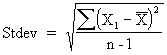
|
The standard deviation is the root-mean-square of a sample. |

See References. |

|
The observation is the total number of values in a sample. |
None |

|
The summation is the total of all the values in a sample. |
None |

|
The minimum is the smallest value in the sample. |
None |
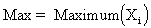
|
The maximum is the largest value in the sample. |
None |
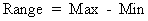
|
The range is the largest value minus the smallest value in the sample. |
None |
|
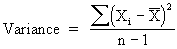
The variance is the square of the standard deviation. |

See References. |

|
The standard error of the mean is the standard deviation of the mean. It measures the extent to which a sample mean can be expected to vary. |

See References. |
|
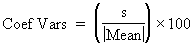
The coefficient of variation is the standard deviation of a sample expressed as a percentage of the mean. It is a measure of relative dispersion. |
See References. |
|
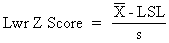
The lower Z-score is the number of standard deviations that the lower specification limit (LSL) is from the mean. |
None |
|
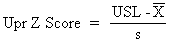
The upper Z-score is the number of standard deviations that the upper specification limit (USL) is from the mean. |
None |
|
Lwr 3 sigma = deviate at probability 0.00135 |
The lower 3 sigma represents three standard deviations from left of the mean. |
None |
|
Upr 3 sigma = deviate at probability 0.99865 |
The upper 3 sigma represents three standard deviations from right of the mean. |
None |
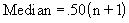
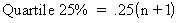
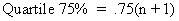
Quality calculates the twenty-fifth, fiftieth, (also referred to as the median), and seventy-fifth quartiles. The quartiles can be displayed as values and are used to graph the Box and Whisker plots.
To compute the quartiles, the system:
Arranges data in ascending order.
Ranks the data accordingly (1 to n).
Multiplies each quartile by n+1.
If the result is an integer, sets the quartile to the value of the calculated rank.
The following table shows quartile equations:
|
Equation |
Statistic |
|---|---|
|
The median is the center or middle of a sample. It is the value above which there are as many values as there are below it. It is also the fiftieth percentile of the sample (Quartile 50 percent). See References. |
|
The twenty-fifth percent quartile is the point separating the lower 25 percent of the values from the upper 75 percent. See References. |
|
The seventy-fifth percent quartile is the point separating the upper 25 percent of the values from the lower 75 percent. |
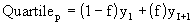
where: p is the percentile, f is the fractional portion of the computed rank, I is the integer portion of the computed rank. |
To resolve calculated values that are not integers (for example, if the percentage lies between two values), the value is interpolated by calculating the weighted average between the two ranks. See References. |
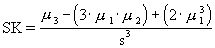
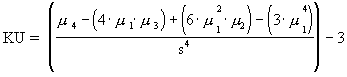
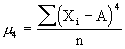
The calculations for skewness and kurtosis use the following examples:
|
Equation |
Statistic |
|---|---|
|
Skewness measures the degree of asymmetry in a sample. |
|
Kurtosis measures the degree of peakedness in a sample. |

|
N/A |

|
N/A |

|
N/A |
|
N/A |
Process capability indices are industrial-accepted calculations for comparing the process output to defined specification limits. For a normal distribution, the process output is defined as :

standard deviations from the mean. For non-normal distributions, Quality determines the Best-Fit Pearson distribution and calculates equivalent 99.73 percent deviations (at 0.00135 and 0.99865).
The following table shows equations that relate to process capability:
|
Equation |
Statistic |
|---|---|
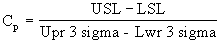
|
The process potential is the ratio of the process distribution to specification limits. It is the potential capability if the process was perfectly centered. This equation requires both upper and lower specifications. |
|
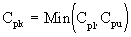
This equation represents the actual process capability. These equations account for shifts in the process center. The 
is the lower of the 
or 
values, or worst-case capability. In the case of a unilateral specification, the 
is set to the calculated 
or 
value. |
|
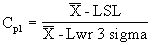
The lower process capability represents the process's ability to perform at the LSL. This equation requires an LSL. |
|
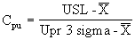
The upper process capability represents the process's ability to perform at the USL. This equation requires a USL. |
where: 
|
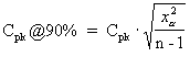
The 90 percent confident Cpk is an adjusted Cpk based on a 90 percent confidence. The result is heavily affected by the sample size. The larger the sample size, the closer the computed value is to the actual Cpk. See References. |

|
The capability ratio is the percentage that the process distribution consumes of the specification. This equation requires both upper and lower specifications. |
where: 
is the area under the curve from the mean to the LSL. |
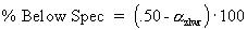
The percent below specification is the estimated area under the curve to the left of the LSL. This equation requires an LSL. |
where: 
is the area under the curve from the mean to the LSL. |
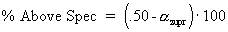
The percent above specification is the estimated area under the curve to the right of the USL. This equation requires a USL. |

|
The total percent out of specification is the total estimated area under the curve outside of the specification limits. |
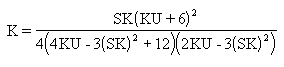
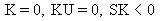
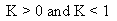
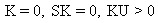
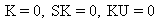
Quality uses Pearson criteria to determine the best-fit distribution for the sample. A K value, computed using the following equation, classifies the distribution as one of the following types:
Pearson Frequency Curves
The following table describes Pearson frequency curves.
|
Type |
Description |
Criteria |
|---|---|---|
|
1 |
Beta |

|
|
2 |
Uniform |
|
|
3 |
Gamma |
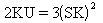
|
|
4 |
Non Central t |
|
|
5 |
Inverse Gamma |

|
|
6 |
Inverse Beta |

|
|
7 |
Student t |
|
|
8 |
Normal |
|
|
10 |
Exponential |
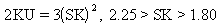
|
Attribute statistics only apply to discrete data types, that is, count data. This type of data is typically associated with defect tallies.
The following table describes equations used with attribute statistics:
|
Equation |
Statistic |
Alternate Equation Forms |
|---|---|---|
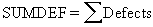
|
The sum of defects is the total count of all the defects in a sample. |
None |
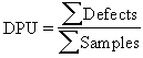
|
This equation represents the average number of defects per unit. |

|
|
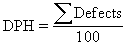
This equation represents the number of defects per 100 units. |
None |
|
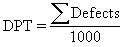
This equation represents the number of defects per 1000 units. |
None |

|
This equation represents the number of defects per million units. |
None |